Gradients, Backprop, and Derivatives in Tensorflow [Draft]

Finding the gradient of¶

$f(x,y) = \\cos{x}\*\\sin{y} + \\frac{x}{y}$

Using Numpy, Autograd, and Tensorflow¶

In [76]:

#Dependencies 
import tensorflow as tf
from mpl_toolkits import mplot3d
import numpy as np
import matplotlib.pyplot as plt
%matplotlib inline

In [126]:

import autograd.numpy as np  # Thinly wrapped version of numpy
from autograd import grad

def f(x, y):
    return np.sin(np.sqrt(x ** 2 + y ** 2))

f_grad = grad(f)  # magic: returns a function that computes the gradient of f

x = 2.
y = 0.

print (f(x, y))
print (f_grad(x, y))

0.9092974268256817
-0.4161468365471424

In [122]:

# Graph 

def f(x, y):
    return np.sin(np.sqrt(x ** 2 + y ** 2))


x = np.linspace(0, 6, 30)
y = np.linspace(-6, 6, 30)

X, Y = np.meshgrid(x, y)

Z = f(X, Y)
fig = plt.figure()
ax = plt.axes(projection='3d')
ax.contour3D(X, Y, Z, 50, cmap='binary')
# ax.set_xlabel('x')
# ax.set_ylabel('y')
# ax.set_zlabel('z')
ax.set_xlabel('X axis')
ax.set_ylabel('Y axis')
ax.set_zlabel('Z axis')

ax = plt.axes(projection='3d')
ax.plot_surface(X, Y, Z, rstride=1, cstride=1,cmap='viridis',edgecolor='none')

Out[122]:

<mpl_toolkits.mplot3d.art3d.Poly3DCollection at 0xb1f8b4cc0>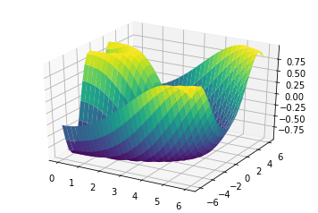

In [125]:

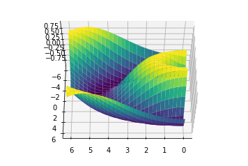
ax.view_init(60, 90)
fig

Out[125]:

In [127]:

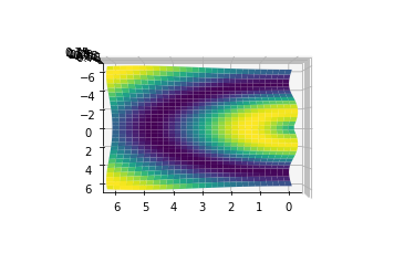
ax.view_init(90, 90)
fig

Out[127]:

In [ ]:

# Computing gradients with some Numpy

# Method 1: Using Partial Derivatives

# def f(x, y):
#     return np.cos(x)*np.sin(y)+(x/y)

# # Compute f(x,y) = cos(x)*sin(x)+(x/y)
# x = input()
# y = input()

# # Forward pass
# w5 = np.cos(x)*np.sin(y)+(x/y) # Node 1
# w6 = (x/y)                     # Node 2

# # Backward pass
# dw7_d
# df_dq = z          # Node 2 input
# df_dz = q          # Node 2 input
# df_dx = 2 * df_dq  # Node 1 input
# df_dy = 1 * df_dq  # Node 1 input

# grad = np.array([df_dx, df_dy, df_dz])

# print f
# print grad

Using tf.gradient to find derivatives¶

In [59]:

%matplotlib inline
import tensorflow as tf
import numpy as np
from math import pi
import matplotlib.pyplot as mp

tf.reset_default_graph()

# Length of graph
length = np.linspace(0,pi*2,100)

# Point at which we want to find derivative at
x = tf.placeholder(tf.float32)

# Function
y=(1/tf.sqrt(x))*(tf.cos(x)*tf.sin(x))


# Running tf session
with tf.Session() as session:
    dy  = session.run(y,feed_dict={x:length})
    grad_out = session.run(tf.gradients(y,x),feed_dict={x:length})
    print("Enter input number")
    input_number = float(input())
    print("Done inputting number")
    grad_at = session.run(tf.gradients(y,x),feed_dict={x:input_number})
    print(grad_at)
    y_at = (1/np.sqrt(input_number))*(np.cos(input_number)*np.sin(input_number))
    x_at = input_number
    print(y_at)
    print(x_at)
    function = grad_at*(length - x_at) + y_at
    writer = tf.summary.FileWriter('logs', session.graph)
    writer.close()

    
mp.plot(length, function, '-r')
mp.plot(length,dy)
mp.plot(length,grad_out[0])

Enter input number
4.1
Done inputting number
[-0.19582547]
0.23229685332631406
4.1

Out[59]:

[<matplotlib.lines.Line2D at 0xb23471a20>]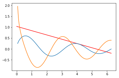

Graph of f(x), F(x), and tan line to f(x) at inputted point¶

Blue line is f(x)¶

Orange line is F(x)¶

Red line is f(x) at indicated point¶

Image unavailable in the recovered copy

Tensorboard of this computational graph¶

One thing to point out: there are two gradients being computed. This is because I computed the gradient twice for graphing and for the tan line. Obviously I could fix this, but the code could be easier for some to understand if the gradient is computed twice.